Moderation
The Conceptual Model
Version 1
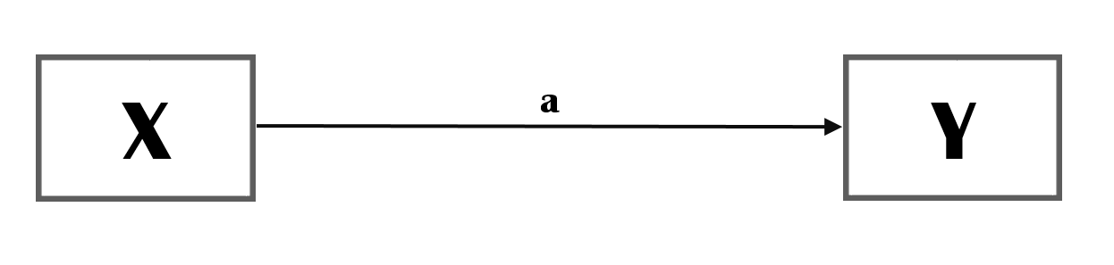
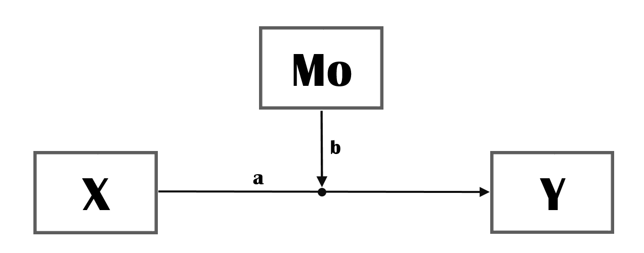
Figure 1: Moderation
The moderator Mo moderates the strength of the impact of X on Y (i.e. path a).
Version 2
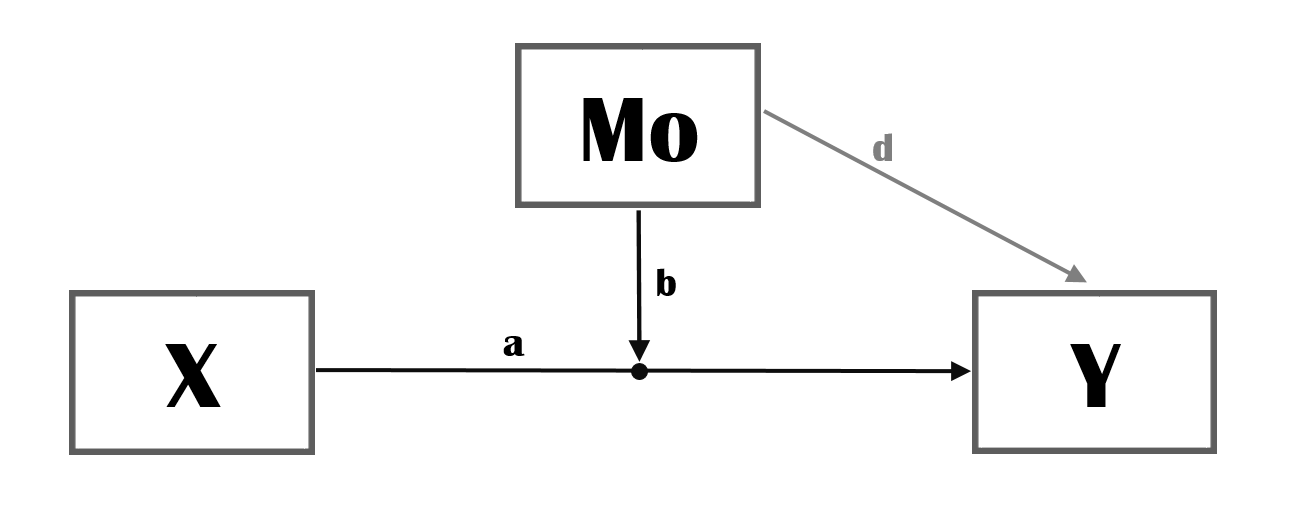
Figure 2: Moderation (including direct effect of moderator)
In Version 2, the direct effect of the Moderator Mo on Y is also drawn. You may not have theorized an effect of Mo on Y and it thus not always necessary to draw this relationship but it is a good idea to consider whether this relationship may exist. When testing for the moderation effect b it is good practice for the direct of of the Moderator (path d) as it will facilitate the interpretation of the moderation effect.
Version 3
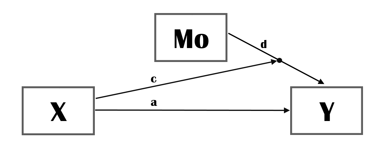
Figure 3: Moderation (equivalent to version 2)
Version 2 and Version 3 are (mathematically) equivalent (structural) models. They will lead to exactly the same model fit. However, from a theoretical viewpoint they are different. (see also examples below).
Version 4
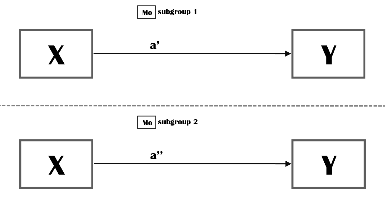
Figure 4: Moderation (categorical Moderator)
If your Moderator is a nominal variable (e.g. gender) it may be more informative for a reader to graphically summarize the model for each category (e.g. men, women, other) separately. This may be especially useful if your model is more complex and includes more independent variables and or mediation variables and you expect more than one relationship to differ depending on gender.1
Explanation
In a conceptual model, the concepts are normally placed in a rectangular. We have three concepts, X, Mo and Y.
We assume an association between X and Y.
The strength of this relation may depend on Mo, the strength of this relation is conditional on the value of Mo. We also call this an interaction effect.
If you want to graphically depict a moderation, it may be useful to show the model without the moderator as well but this is a bit a matter of taste. I have noticed that journal article reviewers and committees that evaluate grant proposals are not always familiar with a graphical depiction of an interaction effect. I have received (more than once!) the comment that my figure was presumably wrong because an arrow was pointing at a different arrow. I therefore now add a very small bullit on the arrow which, I hope, makes clear that it is by design that I point one arrow to another arrow.
It is not always necessary to label the paths but for this tutorial it will turn out to be handy. Normally, when there is no sign (or label) it is assumed that the path has a positive valence. It is, however, good practice to include the valence of the paths in your conceptual models.
Abstract hypotheses
See Version 1/2 above.
positive main effect, positive interaction
- Hypo1: more X leads to more Y (\(a>0\)).
- Hypo2: The relationship between X and Y becomes stronger when Mo increases (\(b>0\)).
positive main effect, negative interaction
- Hypo1: more X leads to more Y (\(a>0\)).
- Hypo2: The relationship between X and Y becomes weaker when Mo increases (\(b<0\)).
negative main effect, positive interaction
- Hypo1: more X leads to less Y (\(a<0\)).
- Hypo2: The negative relationship between X and Y becomes weaker when Mo increases (\(b>0\)).
negative main effect, negative interaction
- Hypo1: more X leads to less Y (\(a<0\)).
- Hypo2: The negative relationship between X and Y becomes stronger when Mo increases (\(b<0\)).
Real life example
X is educational success
Mo is age.
Y is health
- Hypo1: Educational success is (positively) related to a better health.
- Hypo2: The positive relationship between educational success and a better health is stronger for older persons.
Alternatively, one could also formulate just the interaction effect:
- Hypo3: The relationship between educational success and a better health is stronger for older persons.
For hypothesis 3 it is not necessary that there is also a main effect of education on health. Also, the direction of the interaction effect is left a bit implicit (presumably positive). But cannot be falsified when:
- there is no main effect and we observe an interaction effect (regardless of sign)
- there is a positive main effect and a positive interaction effect.
- there is a negative main effect and a negative interaction effect.
For this reason, I would prefer hypotheses 1 and 2 above the single hypothesis 3.
Please compare the following set of hypotheses:
- Hypo1: Educational success is (positively) related to a better health.
- Hypo2: Age is (negatively) related to a better health.
- Hypo3a: The positive relationship between educational success and a better health is stronger for older persons.
and:
- Hypo1: Educational success is (positively) related to a better health.
- Hypo2: Age is (negatively) related to a better health.
- Hypo3b: The negative relationship between age and a better health is weaker for higher educated persons.
Both sets will lead to the same structural equations. But do you think that for older persons education based inequality in health will be more pronounced or that for higher educated age based inequality in health will be less pronounced?
Structural equations
- $ Y= b_0 + b_1X + b_2Mo + b_3XMo Y= b_0 + (b_1 + b_3Mo)X + b_2Mo $
Interpretation (linear model)
The interaction effect is the cross-partial derivative of Y with respect to X and M0:2
\[ \frac{\partial ^2(Y|X,Mo)}{\partial X \partial Mo} = \frac{\partial(b_1 + b_3Mo)}{ \partial Mo} = b_3 \]
Thus the interaction effect is \(b_3\).
Interpretation (non-linear (logit) model)
However, if we have a binary outcome variable our hypotheses are about the probability that Y is 1 (\(P(Y=1)\)). If we estimate the model with a logit function, this is:3
\(P(Y=1|X,Mo)= \frac{e^{(b_0 + b_1X + b_2Mo + b_3XMo)}} {1 + e^{(b_0 + b_1X + b_2Mo + b_3XMo)}} = \frac{1}{1 + e^{-(b_0 + b_1X + b_2Mo + b_3XMo)}}\)
let us define \(P(Y=1|X,Mo)\) as \(F(Y)\) (i.e. the logistic distribution function).
The interaction effect then becomes:
\[ \frac{\partial ^2 F(Y)}{\partial X \partial Mo} = \frac{\partial(f(Y)(b_1 + b_3Mo))}{ \partial Mo} = f(Y)b_3 + f'(Y)(b_1 + b_3Mo)(b_2 + b_3X), \] where \(f(Y)\) is the derivative of the logistic distribution function (i.e. the logistic density function) and \(f'(Y)\) the derivative of the density function with respect to Y.
For more background reading see Norton, Wang, and Ai (2004).
For now we have three take home messages!:
- even if \(b_3\) is non significant you may have a significant interaction effect (namely: \(f'(Y)b_1b_2\)
- the strength, valence (and significance) of the interaction effect depends on the value of \(Y\) (i.e. the covariates), \(b_1\), \(b_2\) and \(b_3\).
- To make sense of interaction effects in nonlinear models, use (3D) plots of predicted values against values of X and Mo!
Lavaan syntax
Following the syntax of the R package Lavaan
- Y~1
- Y~a*X
- Y~d*Mo
- Y~b*X:Mo
Formal test of hypotheses
Load the NELLS data.
rm(list = ls())  #empty environment
require(haven)
nells <- read_dta("../static/NELLS panel nl v1_2.dta")  #change directory name to your working directory
Operationalize concepts. Please note that I mean center the covariates for ease of interpretation!
# We will use the data of wave 2.
nellsw2 <- nells[nells$w2cpanel == 1, ]

# As an indicator of occupational success we will use income in wave 2.
table(nellsw2$w2fa61, useNA = "always")
attributes(nellsw2$w2fa61)
# recode (I will start newly created variables with cm from conceptual models)
nellsw2$cm_income <- nellsw2$w2fa61
nellsw2$cm_income[nellsw2$cm_income == 1] <- 100
nellsw2$cm_income[nellsw2$cm_income == 2] <- 225
nellsw2$cm_income[nellsw2$cm_income == 3] <- 400
nellsw2$cm_income[nellsw2$cm_income == 4] <- 750
nellsw2$cm_income[nellsw2$cm_income == 5] <- 1250
nellsw2$cm_income[nellsw2$cm_income == 6] <- 1750
nellsw2$cm_income[nellsw2$cm_income == 7] <- 2250
nellsw2$cm_income[nellsw2$cm_income == 8] <- 2750
nellsw2$cm_income[nellsw2$cm_income == 9] <- 3250
nellsw2$cm_income[nellsw2$cm_income == 10] <- 3750
nellsw2$cm_income[nellsw2$cm_income == 11] <- 4250
nellsw2$cm_income[nellsw2$cm_income == 12] <- 4750
nellsw2$cm_income[nellsw2$cm_income == 13] <- 5250
nellsw2$cm_income[nellsw2$cm_income == 14] <- 5750
nellsw2$cm_income[nellsw2$cm_income == 15] <- 6500
nellsw2$cm_income[nellsw2$cm_income == 16] <- 7500
nellsw2$cm_income[nellsw2$cm_income == 17] <- NA
# let us scale the variable a bit and translate into income per 1000euro
nellsw2$cm_income <- nellsw2$cm_income/1000

# from household income to personal income
attributes(nellsw2$w2fa62)
table(nellsw2$w2fa62, useNA = "always")
nellsw2$cm_income_per <- nellsw2$w2fa62
nellsw2$cm_income_per[nellsw2$cm_income_per == 1] <- 0
nellsw2$cm_income_per[nellsw2$cm_income_per == 2] <- 10
nellsw2$cm_income_per[nellsw2$cm_income_per == 3] <- 20
nellsw2$cm_income_per[nellsw2$cm_income_per == 4] <- 30
nellsw2$cm_income_per[nellsw2$cm_income_per == 5] <- 40
nellsw2$cm_income_per[nellsw2$cm_income_per == 6] <- 50
nellsw2$cm_income_per[nellsw2$cm_income_per == 7] <- 60
nellsw2$cm_income_per[nellsw2$cm_income_per == 8] <- 70
nellsw2$cm_income_per[nellsw2$cm_income_per == 9] <- 80
nellsw2$cm_income_per[nellsw2$cm_income_per == 10] <- 90
nellsw2$cm_income_per[nellsw2$cm_income_per == 11] <- 100
nellsw2$cm_income_per[nellsw2$cm_income_per == 12] <- NA

nellsw2$cm_income_ind <- nellsw2$cm_income * nellsw2$cm_income_per/100

# as an indicator of educational success we will use highest completed level of education in years.
# the rationale behind this coding this I will take the maximum for university as 16.5 (taking into
# account that some masters are 2 years and some 1 year) and subsequently subtract the years needed
# to obtain a university degree given the degree under consideration.

attributes(nellsw2$w2fa102)
table(nellsw2$w2fa102, useNA = "always")
nellsw2$cm_education <- nellsw2$w2fa102
nellsw2$cm_education[nellsw2$w2fa102 == 1] <- 6
nellsw2$cm_education[nellsw2$w2fa102 == 2] <- 9
nellsw2$cm_education[nellsw2$w2fa102 == 3] <- 10
nellsw2$cm_education[nellsw2$w2fa102 == 4] <- 11
nellsw2$cm_education[nellsw2$w2fa102 == 5] <- 12
nellsw2$cm_education[nellsw2$w2fa102 == 6] <- 10
nellsw2$cm_education[nellsw2$w2fa102 == 7] <- 11
nellsw2$cm_education[nellsw2$w2fa102 == 8] <- 14
nellsw2$cm_education[nellsw2$w2fa102 == 9] <- 15
nellsw2$cm_education[nellsw2$w2fa102 == 10] <- 16.5
nellsw2$cm_education[nellsw2$w2fa102 == 11] <- 16.5
nellsw2$cm_education[nellsw2$w2fa102 == 12] <- 7
nellsw2$cm_education[nellsw2$w2fa102 == 13] <- 11
nellsw2$cm_education[nellsw2$w2fa102 == 14] <- 14.5
nellsw2$cm_education[nellsw2$w2fa102 == 15] <- 4


# mean centering
nellsw2$cm_education_c <- nellsw2$cm_education - mean(nellsw2$cm_education, na.rm = T)
nellsw2$cm_age_c <- nellsw2$w1cage - mean(nellsw2$w1cage, na.rm = T)

# define a dichotemous moderator based on age.
nellsw2$cm_old_d <- ifelse(nellsw2$cm_age_c >= 0, 1, 0)


# as an indicator of health we will use subjective well being from 5 (excellent) to 1 (bad) thus we
# have to reverse code original variable
attributes(nellsw2$w2scf1)
table(nellsw2$w2scf1, useNA = "always")
nellsw2$cm_health <- 6 - nellsw2$w2scf1
##
## 1 2 3 4 5 6 7 8 9 10 11 12 13 14 15 16 17 <NA>
## 55 78 103 204 338 326 282 272 276 205 133 62 48 22 22 29 374 0
## $label
## [1] " wat is het netto inkomen per maand van u en uw partner samen?/van u?/ "
##
## $format.stata
## [1] "%8.0g"
##
## $labels
## Minder dan ¤150 per maand ¤150 - ¤299 per maand ¤300 - ¤499 per maand
## 1 2 3
## ¤500 - ¤999 per maand ¤1.000 - ¤1.499 per maand ¤1.500 - ¤1.999 per maand
## 4 5 6
## ¤2.000 - ¤2.499 per maand ¤2.500 - ¤2.999 per maand ¤3.000 - ¤3.499 per maand
## 7 8 9
## ¤3.500 - ¤3.999 per maand ¤4.000 - ¤4.499 per maand ¤4.500 - ¤4.999 per maand
## 10 11 12
## ¤5.000 - ¤5.499 per maand ¤5.500 - ¤5.999 per maand ¤6.000 - ¤6.999 per maand
## 13 14 15
## ¤7.000 of meer per maand weet niet, wil niet zeggen
## 16 17
##
## $class
## [1] "haven_labelled" "vctrs_vctr" "double"
##
## $label
## [1] " hoe groot is uw bijdrage in dit inkomen ongeveer? kunt u een percentage noemen "
##
## $format.stata
## [1] "%8.0g"
##
## $labels
## vrijwel geen bijdrage ongeveer 10% ongeveer 20% ongeveer 30%
## 1 2 3 4
## ongeveer 40% ongeveer 50% ongeveer 60% ongeveer 70%
## 5 6 7 8
## ongeveer 80% ongeveer 90% ongeveer 100% weet niet
## 9 10 11 12
##
## $class
## [1] "haven_labelled" "vctrs_vctr" "double"
##
##
## 1 2 3 4 5 6 7 8 9 10 11 12 <NA>
## 253 48 89 259 233 242 183 229 114 63 887 229 0
## $label
## [1] " wat is uw hoogst voltooide opleiding, dat wil zeggen waarvan u een diploma heef"
##
## $format.stata
## [1] "%8.0g"
##
## $labels
## lagere school
## 1
## lbo, vmbo-kb\\bbl
## 2
## mavo, vmbo-tl
## 3
## havo
## 4
## vwo\\gymnasium
## 5
## mbo-kort (kmbo), primair leerlingwezen, bol\\bbl niveau 1 of
## 6
## mbo-tussen\\lang (mbo), secundair\\tertiar leerlingwezen, bol\\
## 7
## hbo
## 8
## universiteit (bachelor)
## 9
## universiteit (master, doctoraal)
## 10
## promotietraject
## 11
## buitenlandse opleiding, niet goed in te delen, lager onderwi
## 12
## buitenlandse opleiding, niet goed in te delen, middelbaar on
## 13
## buitenlandse opleiding, niet goed in te delen, hoger onderwi
## 14
## geen opleiding
## 15
##
## $class
## [1] "haven_labelled" "vctrs_vctr" "double"
##
##
## 1 2 3 4 5 6 7 8 9 10 11 12 13 14 15 <NA>
## 118 223 202 205 117 223 737 586 89 208 12 8 20 17 34 30
## $label
## [1] " wat vindt u, over het algemeen genomen, van uw gezondheid? "
##
## $format.stata
## [1] "%8.0g"
##
## $labels
## uitstekend zeer goed goed matig slecht
## 1 2 3 4 5
##
## $class
## [1] "haven_labelled" "vctrs_vctr" "double"
##
##
## 1 2 3 4 5 <NA>
## 438 853 1211 247 48 32And test the model with Lavaan.
Interaction variable approach
require(lavaan)

model <- "
  #structural model
  cm_health~ a*cm_education_c + d*cm_age_c + b*cm_education_c:cm_age_c
  #intercepts
  cm_health~1
  cm_education_c ~1
  cm_age_c~1

  #residual variance
  cm_health ~~ cm_health

  #variances
  cm_education_c ~~ cm_age_c
"


fit <- lavaan(model, data = nellsw2, auto.var = T, meanstructure = T)
summary(fit, standardized = TRUE)
## lavaan 0.6-7 ended normally after 31 iterations
##
## Estimator ML
## Optimization method NLMINB
## Number of free parameters 11
##
## Used Total
## Number of observations 2767 2829
##
## Model Test User Model:
##
## Test statistic 130.504
## Degrees of freedom 3
## P-value (Chi-square) 0.000
##
## Parameter Estimates:
##
## Standard errors Standard
## Information Expected
## Information saturated (h1) model Structured
##
## Regressions:
## Estimate Std.Err z-value P(>|z|) Std.lv Std.all
## cm_health ~
## cm_edctn_c (a) 0.054 0.007 8.266 0.000 0.054 0.152
## cm_age_c (d) -0.019 0.002 -10.558 0.000 -0.019 -0.194
## cm_dct_:__ (b) 0.002 0.001 2.130 0.033 0.002 0.039
##
## Covariances:
## Estimate Std.Err z-value P(>|z|) Std.lv Std.all
## cm_education_c ~~
## cm_age_c -0.131 0.448 -0.292 0.770 -0.131 -0.006
##
## Intercepts:
## Estimate Std.Err z-value P(>|z|) Std.lv Std.all
## .cm_health 3.495 0.017 207.350 0.000 3.495 3.816
## cm_education_c 0.002 0.049 0.039 0.969 0.002 0.001
## cm_age_c -0.065 0.174 -0.375 0.708 -0.065 -0.007
## cm_dctn_c:cm__ 0.000 0.000 0.000
##
## Variances:
## Estimate Std.Err z-value P(>|z|) Std.lv Std.all
## .cm_health 0.786 0.021 37.195 0.000 0.786 0.937
## cm_education_c 6.626 0.178 37.195 0.000 6.626 1.000
## cm_age_c 83.937 2.257 37.195 0.000 83.937 1.000
## cm_dctn_c:cm__ 479.911 12.902 37.195 0.000 479.911 1.000We observe that higher educated persons report higher SWB.
We observe that older persons report lower SWB.
We observe that the relationship between education and SWB is higher for older persons.
multigroup approach
require(lavaan)
# no equality constraints across groups whatsoever.
model <- "
  #structural model
  cm_health~ c(a1,a0)*cm_education_c #I am giving the education effects specific names for each group
  #intercepts
  cm_health~1

  #residual variance
  cm_health ~~ cm_health

  #test for difference
  a1a0:=a1-a0
"


fit <- lavaan(model, data = nellsw2, auto.var = T, meanstructure = T, group = "cm_old_d")
summary(fit, standardized = TRUE)
## lavaan 0.6-7 ended normally after 15 iterations
##
## Estimator ML
## Optimization method NLMINB
## Number of free parameters 6
##
## Number of observations per group: Used Total
## 1 1530 1572
## 0 1237 1257
##
## Model Test User Model:
##
## Test statistic 0.000
## Degrees of freedom 0
## Test statistic for each group:
## 1 0.000
## 0 0.000
##
## Parameter Estimates:
##
## Standard errors Standard
## Information Expected
## Information saturated (h1) model Structured
##
##
## Group 1 [1]:
##
## Regressions:
## Estimate Std.Err z-value P(>|z|) Std.lv Std.all
## cm_health ~
## cm_dctn_c (a1) 0.066 0.008 7.895 0.000 0.066 0.198
##
## Intercepts:
## Estimate Std.Err z-value P(>|z|) Std.lv Std.all
## .cm_health 3.353 0.023 146.715 0.000 3.353 3.677
##
## Variances:
## Estimate Std.Err z-value P(>|z|) Std.lv Std.all
## .cm_health 0.799 0.029 27.659 0.000 0.799 0.961
##
##
## Group 2 [0]:
##
## Regressions:
## Estimate Std.Err z-value P(>|z|) Std.lv Std.all
## cm_health ~
## cm_dctn_c (a0) 0.038 0.011 3.549 0.000 0.038 0.100
##
## Intercepts:
## Estimate Std.Err z-value P(>|z|) Std.lv Std.all
## .cm_health 3.675 0.025 145.563 0.000 3.675 4.120
##
## Variances:
## Estimate Std.Err z-value P(>|z|) Std.lv Std.all
## .cm_health 0.788 0.032 24.870 0.000 0.788 0.990
##
## Defined Parameters:
## Estimate Std.Err z-value P(>|z|) Std.lv Std.all
## a1a0 0.028 0.014 2.083 0.037 0.028 0.097We observe that the relationship between education and SWB is significantly higher for older persons.
References
Norton, Edward C, Hua Wang, and Chunrong Ai. 2004. “Computing Interaction Effects and Standard Errors in Logit and Probit Models.” The Stata Journal 4 (2): 154–67.