Small worlds

A complete, full, or sociocentric network is a network within a sampled context or foci of which we know all nodes and all connections between nodes. The boundaries of the network are thus a priori defined and the contexts in which nodes are present are the sampled units. We may for example sample a classroom, neighborhood, university or country and collect all relations between all nodes within this context.

Now, suppose we live in a world, called “Smallworld”, of 105 persons (a small world indeed) and have information on all friendship (or trust) relations between its citizens. How would such a network look like? Well it turns out that (large) social networks of positive relations often have a specific structure. And this structure is called A Small World. Lets have a look at the small world structure of SmallWorld.

Play with the small world network of Smallworld. Zoom in and out, turn it around and click on some nodes. How would you describe the structure of the network in Smallworld. Well, I would describe it as a network with a: (1) relatively low density; (2) relatively high degree of clustering and (3) a relatively low average degree of separation (or path length). These three characteristics are defining features of small world networks. But what does density, clustering and path length mean?, and what do we mean with ‘relatively’, that does not sound very scientific does it?!

Density

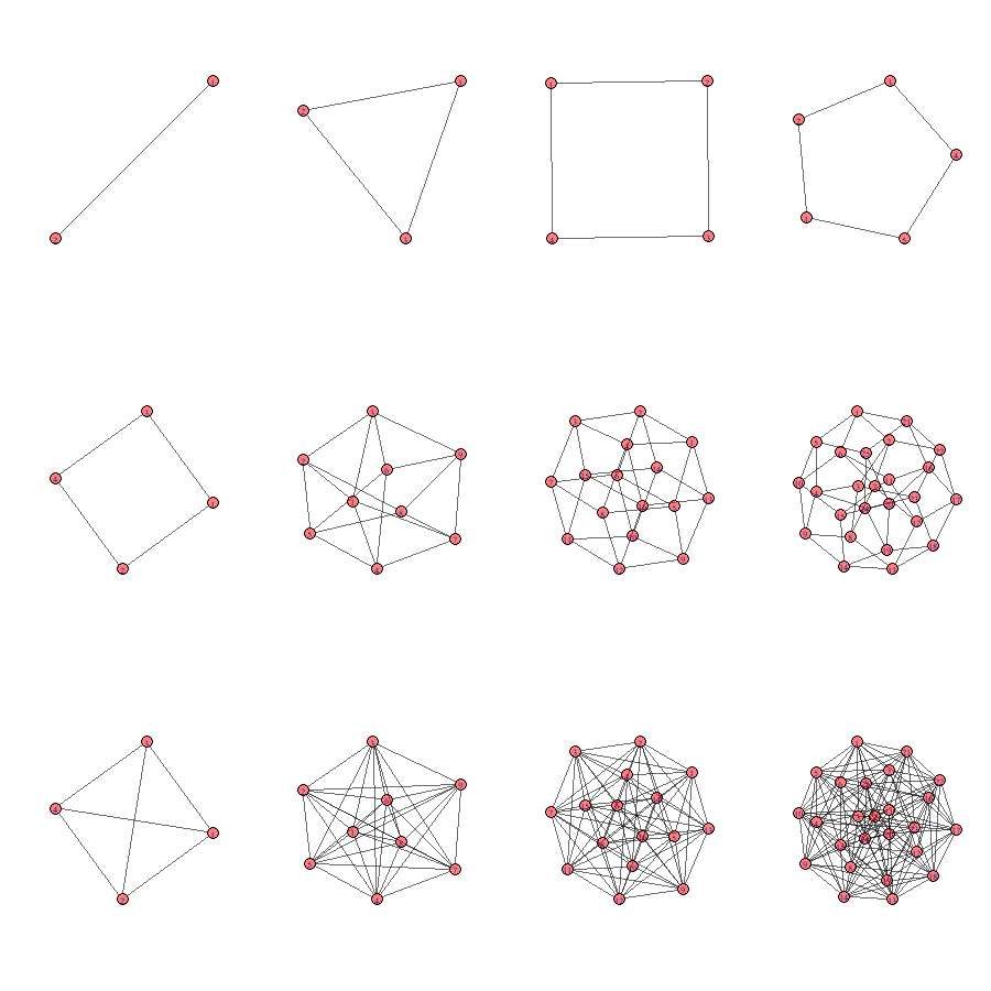
Density is defined as all observed relations divided by all possible relations. Look at the examples below. Are you able to calculate the density of the networks yourself?

The density in Smallworld turns out to be 0.14. For comparison, if we look at friendship networks among pupils in classrooms, we generally observe a density within the range of .2 and .4.

Centrality

Closely related to density is the concept of degree. The number of ingoing (indegree), outgoing (outdegree) or undirected (degree) relations from each node. In real social networks, we generally observe a right-skewed degree distribution (most people have some friends, few people have many friends). In Smallworld the nodes either have 14 or 15 relations, a very uniform and thus unrealistic degree distribution.

People in a network with relatively many degree are called more central and (normalized) degree centrality is formally defined as:

$$ C_D(v_i) = \frac{deg(v_i) - min(deg(v))} {max(deg(v)) - min(deg(v))}, $$

where $ C_D(v_i) $ is degree centrality of $ v_i $, vertex i, and ‘deg’ stands for ‘degree’. $ max(deg(v)) $ is the maximal observed degree. $ min(deg(v)) $ is the minimal observed degree.¹

Closely related to degree centrality is (normalized) ‘closeness centrality’:

$$ C_C(v_i) = \frac{N}{\sum_{j}d(v_j, v_i)}, $$

with N the number of nodes and d stands for distance.

A final important measure of centrality is called betweenness. It is defined as:

$$ C_B(v_i) = \frac{\sigma_{v_j,v_k}(v_i)}{\sum_{j\neq k\neq i}\sigma(v_j,v_k)}, $$

where $ \sigma(v_j,v_k) $ is the number of shortest paths between vertices j and k, $ \sigma_{v_j,v_k}(v_i) $, are the number of these shortest paths that pass through vertex $ v_i $ . One way to normalize this measure is as follows:

$$ C_{B_{normalized}}(v_i) = \frac{C_B(v_i) - min(C_B(v))}{max(C_B(v))-min(C_B(v))} $$

Path Length

According to wiki, average shortest path length is defined as the average number of steps along the shortest paths for all possible pairs of network nodes. Thus the length of a path is the number of edges the path contains. Some pairs of nodes (dyads) may not be connected at all. How to deal with those? Well we could calculate the average path length of all connected nodes. See for example the network below.

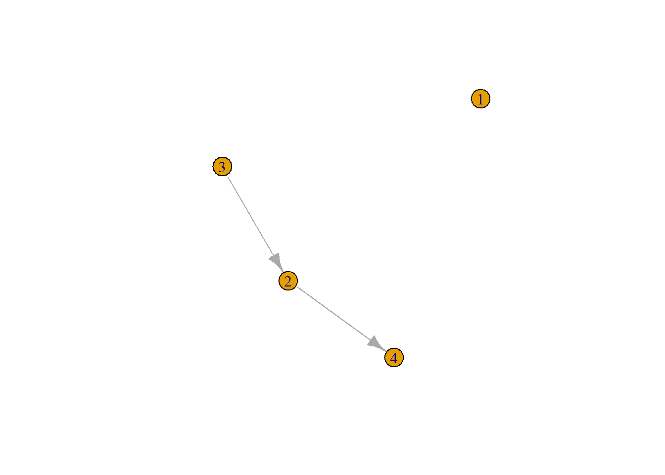This is a directed graph, thus node 3 is connected to node 4 (path length 2) but 4 is not connected to 3. What is the average path length? …
It is: 1.33. The average path length in Smallworld is very low considering the size and density, it is: 2.12. Since path length excludes disconnected nodes, it does not necessarily tells us something about the ‘degrees of separation’. Let us instead calculate for each path length the proportion of nodes each node can reach and take the average value of that.

Thus for the random_graph above, if we take a path length of two we find that nodes 1 to 4 node can reach 0, 0.25, 0.5, 0 of all other nodes, respectively. This makes for an average reach of 0.1875.
For Smallworld we find the following:

• path length one: 0.13%.
• path length two: 0.74%.
• path length three: 0.99%.

We already came across the six-degrees-of-separation phenomenon. This is the observation that for real societies and real worlds 100% of the population would be connected to 100% of the population via 6 other persons (making for a path length of seven); with path length seven, the average reach is 100%.

Clustering

Clustering is an interesting concept. We have immediately an intuitive understanding of it, people lump together in separate groups. But how should we go about defining it more formally? The clustering coefficient for $ v_i $ is defined as the observed ties between all direct neighbors of $ v_i $ divided by all possible ties between all direct neighbors of $ v_i $ . Direct neighbours are connected to $ v_i $ via an ingoing and/or outgoing relation. For undirected networks, the clustering coefficient is the same as the transitivity index (the number of transitive triads divided by all possible transitive triads). For directed graphs not so.
Before we can start calculating the average (or global) clustering index we have to take a decision about what to do with vertices without neighbors. We may set their clustering index to zero and include them, or set them at NaN and exclude them (my preference).
The clustering coefficient of Smallworld is 0.34

Relatively scientific

We stated that in a small world network, despite having a low density and being relatively clustered, the relative average path length is small. What do we mean with relative? Well, in SNA it means that if we would make a random graph, the chance is very low (lower than say 5%) that this graph would have a higher degree of clustering and a shorter average path length. Normally, we do set constraints on these random graphs. In this case that they should have the same size and density as the graph we want to compare. (We could also constrain on the observed degree distribution.) Let us make 1000 random graphs with size 105 (just as in Smallworld) and with a density of 0.14. And let us make a histogram of all observed average degree of clustering and path lengths.

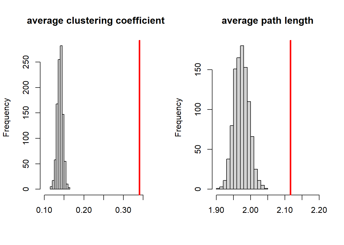
The values of Smallworld are plotted in red. Smallworld indeed has a very high degree of clustering. However, we see that the random graphs have a low average shortest path length and the average path length of Smallworld is actually even relatively high compared to random graphs. Based on these observations we may now calculate the smallworldlyness of Smallworld. One definition is:

$$ \sigma = \frac{C/C_r}{L/L_r}, $$

where C is the average clustering of the observed graph and $ C_ r $ is the clustering of the random graph, L is the average shortest path length of the observed graph and $ L_r $ is the average shortest path length of the random graph. With $ \sigma > 1 $ the network is a small-world network. The smallworldness of Smallworld is 2.16.

This leaves us with just one thing unexplained: relatively low density. Well if we would flip a coin for each possible tie between two random nodes, the density would be 50%. Thus all networks (with binary relations) with a density lower than 50% have a relatively low density. And there you have it: absolute science again.

Literature

Part 1: Causes

Tolsma, J., van Deurzen, I., Stark, T. H., & Veenstra, R. (2013). Who is bullying whom in ethnically diverse primary schools? Exploring links between bullying, ethnicity, and ethnic diversity in Dutch primary schools. Social Networks, 35(1), 51-61.

Stark, T. H. (2015). Understanding the selection bias: Social network processes and the effect of prejudice on the avoidance of outgroup friends. Social Psychology Quarterly, 78(2), 127-150.

Part 2: Consequences

Gremmen, M. C., Dijkstra, J. K., Steglich, C., & Veenstra, R. (2017). First selection, then influence: Developmental differences in friendship dynamics regarding academic achievement. Developmental psychology, 53(7), 1356.

Huitsing, G., Snijders, T. A., Van Duijn, M. A., & Veenstra, R. (2014). Victims, bullies, and their defenders: A longitudinal study of the coevolution of positive and negative networks. Development and psychopathology, 26(3), 645.

Part 3: Methods

Ripley, R.M., Snijders, T.A.B., Boda, Z., Vörös, A. & Preciado, P. (2020). Manual for RSiena (version August 14, 2020). Oxford: University of Oxford, Department of Statistics; Nuffield College.

SELF-TEST

Each chapter ends with a SELF-TEST. Using what you learned in this chapter you should be able to answer both the theoretical and methodological part of this SELF-TEST.